Posted by: @rob-of-york

↑

The HTC value is found by averaging over lots of degree-hours, however, the details of exactly what happens each hour or each day are unnecessary for the calculation (a big advantage in this approach), only the average indoor and outdoor temperatures for the month are needed along with the energy going in from various sources. (Caveat that outdoor temperature is always below indoor).

I get the general principle. My contention is that you need to sample often enough to get true average, since infrequent sampling may miss observations that should contribute to the average, but will be missed out with infrequent sampling, if that makes sense. For example, here are my hourly OAT measurements from the first half of August this year, with two mean daily temperature values (°C), one calculated using hourly samples, the other using two samples, midday and midnight. The differences aren't huge, but they are there nonetheless:

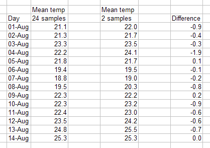
Thus, I suggest, while the HTC can use averages over long periods, those averages do need to be based on enough samples to ensure the average reflects the reality of what actually happened, and that means the data need to be collected at relatively short intervals. In other words, you have to start with hourly samples, even if you end up with a single average covering a whole month.

But I think we agree on this, that is, you need enough underlying samples. All I am doing is emphasising the point that the long term averages used to calculate the HTC must be based on frequent enough underlying sampling to ensure the final averages reflects what actually happened.

The other point is whether you need to calculate the heat delivered from other sources. Given that with a steady IAT, the heat loss = the heat delivered by the primary heat source (boiler, heat pump) + the heat delivered by all the other heat sources (people, electrical appliances, solar gain), then if you measure the heat delivered by the primary heat source, that is it not the case that that value is the amount of heat the primary heat source needs to deliver? 

I'm still working on/thinking about this and I also want to run the HTC method on my Jan 2026 data (I have all the necessary variables) to see what results I get, but have some other things I need to attend to right now. I'll be back later!

Posted by: @jamespa 

Whilst I don't like determining things based on a single measurement point because you don't have a tool to spot errors, I also recognise that you have to use the (best) info you can reasonably get. 

I couldn't agree more with the point about not trusting single measurement points. Best to repeat the calculation over multiple months if possible.

I originally did the calculations for my house based on the Dec-Jan period in 2014/5. If I break it down into separate calculations for Dec-24, Jan-25, and Feb-25, the heat loss works out at 6210W, 6110W, and 6220W respectively, and the HTCs are 259W, 255W, and 259W respectively. Weighted average 6170W and HTC 257W. (The solar gain was based on 10 kWh per sqm incident in Dec and Jan, and 20 kWh incident per sqm in Feb). The average outdoor temperature changed considerably over these three months, 7.3C in Dec, 2.8C in Jan, and 5.0C in Feb. Indoor averages were near constant at 18.5C, 18.2C, and 18.3C. 

Since these figures are all very much in the same ballpark that gives me good confidence that the real heat loss in somewhere in the range 5900W to 6400W. (These are the outliers with the solar gain adjusted +or- 5 kWh per sqm from the defaults. The rest of the data are either measured by the smart meter or good estimates of occupancy, so only a small variability is likely there).

With good quality input data, I think this practical approach is a really good way of getting a handle on heat loss values.

Posted by: @cathoderay 

All I am doing is emphasising the point that the long term averages used to calculate the HTC must be based on frequent enough underlying sampling to ensure the final averages reflects what actually happened.

I completely agree. The average temperatures that I used were based on half-hourly readings from the weather station and its indoor unit. A once or twice a day measurement wouldn't be good enough to get an accurate average.

I looked at data from the nearest historic met office weather station to me, which is about 20 miles away, and it's data gives averages of 6.9C, 2.8C, and 5.0C for Dec, Jan, and Feb 2024/5 compared to the 7.3C, 2.8C, and 5.0C from my own weather station. So the differences are there but not huge. I think using met office data would be plausible to get a ballpark figure for someone who does not have their own outdoor temperature data.

The other point is whether you need to calculate the heat delivered from other sources. Given that with a steady IAT, the heat loss = the heat delivered by the primary heat source (boiler, heat pump) + the heat delivered by all the other heat sources (people, electrical appliances, solar gain), then if you measure the heat delivered by the primary heat source, that is it not the case that that value is the amount of heat the primary heat source needs to deliver? 

If you were only looking at a single data point, i.e. a one value for the difference between outdoor and indoor temperatures then that's right. However, in general its not. While the contribution from other sources in Watts is constant, the percentage contribution to the total required for some temperature difference varies with the temperature difference. For example for a 2 degree difference in temperature, the contribution from other sources may be enough to cover all of the heat required, whereas for a 24 degree difference, it would only cover a 1/12th of it. This means that the calculation doesn't work properly without the energy from other sources included, unless the averages for the month matched exactly the design temperatures (e.g. -3C outside, 21C inside), which they are never going to do.

For example, assume the real HTC value is 250W and 500W are always provided by other sources. Let's say our reference month has an average outdoor temperature of 8C and indoors its 20C, a difference of 12 degrees. Also, let's assume the energy from the heating system works out at 2500W to support that temperature difference. If we ignore the heat delivered from other sources, we calculate the HTC as 2500/12 = 208.333W. If we use that value to obtain the heat loss for a 24 degree temperature difference, we get 5000W, and so it looks like we need a 5kW heat pump. However, the correct HTC is calculated by including the heat from other sources as well as the heating system, which is (500 + 2500)/12 = 250W. Hence the heat loss for a 24 degree temperature difference is 6000W, of which 500W are provided by other sources, hence we actually need a 5.5kW heat pump.

The discussion continues to be interesting and I have only just got back to looking at it (Sunday is cycling and F1 day).

The discussion about measuring tank content continues to be interesting. We have a 2000 litre tank and I have programmed a cylindrical calculation into Excel which allows me to plot volume from a dip stick. The dip stick is calibrated in micrometers so is very accurate. Only joking : it consists or a rusty steel bar which I dunk into the tank and then measure the wet rust using an aged Stanley retractable tape measure. The measurement needs to be quick as the oil otherwise leeches up the rust! So, there's no way to get anything with precision. Given that I spent most of my life measuring things in Mhz and ns and pA and uV, that's a tough pill to swallow! The thing is, I've long since left that world behind and I'm happy to be less precise, but not to be completely wrong!

What is clear is that much of this measuring is far from an exact science - be it the heat loss calculation and significant variability introduced by guestimates from installers, consultants and homeowners while satisfying the demands of MCS and minimising comeback from homeowners if the installation fails to satisfy or the measuring of oil with a rusty dipstick,

Accurate flow meters in the oil line  (which is not the case at my house) would seem to be the only sure way - so this second approach is fraught with issues.

If a 12KW Vaillant will be enough for our house, or even a 15KW Grant will be enough, only time will tell. What I know at the moment is that, "probably", for all but the very coldest of days.

Using @JamesPA formula of dividing KW of energy input by a factor of (I chose) 2300 puts our heat loss somewhere around 11 or 12 (that allows for a contribution from our wood burners in the evenings). That my heat loss calculation as well as that of installer C are in that region and with my lack of confidence in what the consultant (installer B) is suggesting is required, keeps me favouring installer C.

That an installer who advocates a heat loss and corresponding design and then needs to deliver a satisfactory outcome, seems a safer bet than a consultant who comes up with a number and caveats and statements which seem questionable, and then piles the risk on to a nominated external contractor. 

One of the motivations for moving to a heat pump is that we want to add additional emitters in our lounges and, while I could have emitters added and still run them with our oil boiler, I may as well take the Government shilling (well, 108,000 of them, actually) and move off fossil fuels. .... except, if the heat pump fails to keep the house warm on the coldest of days, I'll need to fire up the wood burners and add to global warming!

Thankfully, we have a decent, on our land, source of seasoned wood - I just have to chain saw, split it and dry it. Certainly I would need to cut a fraction of the wood that we have to do now (unless the HP is way under capable) and a wood burner is nice for cosiness , less nice as a necessity.

At least our nearest neighbours are about 50 yards away and most people around here have wood burners or fossil fuel boilers - such is rural ways when there is no gas main!

Thanks again everyone.

@rob-of-york — thanks again for a clear helpful explanation. If I can summarise, I think the key point is that the heat from other sources stays pretty constant, and so as a proportion of the total heat delivered it becomes relatively smaller as the demand increases. Using just the heat delivered by the primary source misses that declining proportion of the heat that comes from others sources. 

I have now done the HTC (hat transfer coefficient) based heat loss assessment based on January of this year for my house, which I can do because I already collect all the relevant variables, apart from the other non-primary heat source variables. These I estimated using @rob-of-york's spreadsheet. Here are the worked calculations. By convention, I refer to the indoor air temperature as the IAT, and the outdoor air temperature as the OAT.

The final formula is heat loss at design temps (what we commonly abbreviate to 'heat loss') = HTC x delta t between IAT and OAT at design temps

For my grant funded installation, the delta t had to be the MCS delta t, in my case OAT -2, IAT 21, delta t 23°C. However in normal day to day use, I aim for a IAT of 19°C, but often overshoot a tiny bit. In January this year, my mean IAT was 19.6°C, so I will use a delta t of 21.6°c. The IAT data is collected once a minute over modbus from a MD02 temperature and humidity sensor in the middle of the ground floor of my house. The data ends up in a minute data csv file, from which the hourly averages are calculated.  

The HTC formula is HTC = energy delivered over the relevant period (one 31 day month in this case) divided by the degree-hours for the same period. In plain English, the HTC is the amount of energy required to 'cover' (achieve) one degree-hour, ie keep the IAT above the OAT by one degree for one hour.

My monitoring system separates out the space heating from the DHW heating. The energy delivered to the house is calculated from the flow/return delta t x flow rate x specific heat capacity of the circulating fluid (which has some glycol in my case), with the first two variables coming from Midea's own data, again over modbus. I have not been able to verify the Midea flow and return temperature values, but I do have an analogue flow meter in the primary circuit, and that suggests the Midea flow rate values are reasonably accurate. The data is collected once a minute, and then summed to get the hourly value. For January of this year, that monthly total was 4612kWh.

The simplified (using the monthly averages, so long as those averages are based on sufficiently large samples, which mine are, being based on once a minute readings) degree-hour formula is degree-hours = (average IAT - average OAT) x 24 (for 24 hours in the day) x 31 (for 31 days in January), because one degree-hour is one degree for one hour, and we want the total number of degree-hours for January. The average OAT was 6.1°C, making the calculation (19.6 - 6.1) x 24 x 31 = 10005 degree-hours.

I then calculate the HTC as 4612 / 10005 = 0.4609 kW/°C, or 461W/°C. This figure is high, because I have an 'old leaky building'. Time 'drops out' because it is in both above and below in the division, so this really is a power (watts) number, rather than an energy number (kWh). 

Returning to the original (final) formula above, this gives me a heat loss at design temps of 0.4609 x 21.6 = 9.95 kW. 

For comparison, here is my previous empirical heat loss assessment, based on plotting hourly energy delivered against hourly mean OAT, using data from Oct to mid-Dec last year (the most recent plot I did):

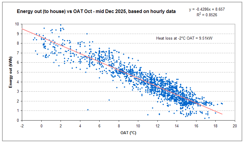
HTC method 9.95 kW, my empirical method 9.51 kW. Close, but not that close. Maybe the different periods (Oct to Mid Dec for my method, Jan for the HTC method) account for the difference?

By the way, I think the gradient of the line is closely related to the HTC; had I used degree-hours rather than OAT on the X axis, I think the gradient may be the HTC.

However, I have not yet allowed for heat from other heat sources in the calculations. These work out at around 320 kWh for 31 days in winter according to @rob-of-york's spreadsheet. The HTC based calculations then become HTC = (4612 + 320) / 10005 = 0.4930, heat loss = 0.4930 x 21.6 = 10.65, of which 0.32 kW come from other sources, leaving a loss of 10.33 kW to be covered by the heat pump. 

I think I have done that other heat sources adjustment correctly, yet it appears to increase the loss to be covered by the heat pump... 

For what it is worth, here is what actually happened in Jan of this year: 

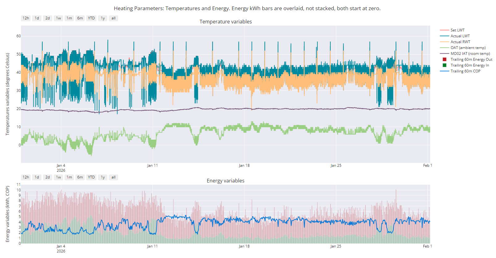
During the cold spell at the beginning of the month, when the OAT briefly went below the design OAT (-4°C OAT on the early morning of 6th Jan), the IAT did drop a little (to 18° against my target of 19°), with the heat pump putting out about 9.5 kWh per hour. This incidentally suggests I may need to tweak the left hand end of my weather compensation curve to accommodate these very low temps when they occur. But it does seem that by and large at around -2° OAT (the design OAT) a delivered heat input of around 9.5 kWh per hour plus the extra 0.32 kWh from other sources just about keeps my IAT where it should be most of the time.

By the way, the Freedom Heat Pump spreadsheet (the one used to size the heat pump at installation time) heat loss was 12.3 kW.  

@cathoderay and others.

I think there may be some confusion over the contributions from external sources creeping in.  They may be a variable proportionn of the heat loss but (with the exception of solar gain) they are essentially a constant absolute value.  Thus they don't figure in the HTC (which is the gradient of loss Vs dt) and have the effect of reducing the amount of heat that the heat pump needs to supply.  When you measure the consumption at any given DT you are measuring loss-fixed contributions (which we might call apparent loss).  This is  htc x dt - fixed contribution and your heat source has to supply that amount only.

If you plot apparent loss(or in principle consumption) Vs DT, the HTC is the gradient and the fixed contribution the intercept at DT=0, which should be negative.

I don't know if that helps or hinders, apologies if the latter.

Posted by: @jamespa

↑

When you measure the consumption at any given DT you are measuring loss-fixed contributions (which we might call apparent loss).  This is  htc x dt - fixed contribution and your heat source has to supply that amount only.

This is the point that I was getting at earlier, when you measure the heat delivered to the house by the primary heat source, the number you get is (a)  what the primary heat source has to supply (given a stable IAT) and (b) is net of the other heat sources. I then sort of persuaded myself that because the other heat sources are relatively fixed (in my case, the biggest component is other electrical appliances, and by and large use of them will remain relatively constant), then they do vary as a proportion of the total heat supplied, as in the greater the total, the smaller the proportion, and somehow this has to be taken into account. Now I am not so sure again!    

Here is my hourly energy delivered vs mean OAT plot (DHW largely excluded) for January 2026, ie the same period used for the HTC calculation. 

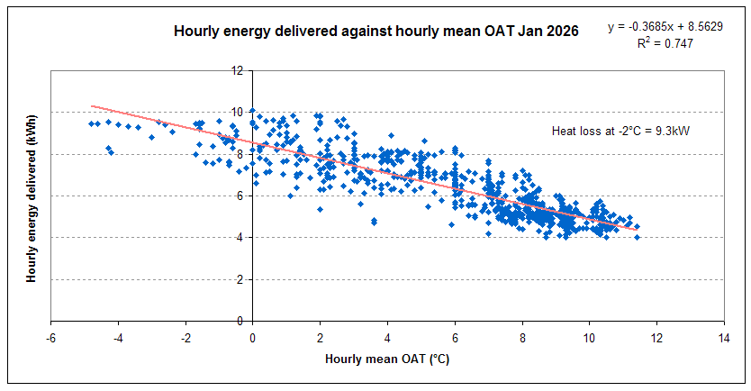
This suggests the heat loss covered by the primary heat source is 9.3 kW, a bit less than the previous estimate (9.51 kW). I think this may be in the range of expected variability. Since this chart is the raw data displayed visually, I by nature tend to give this greater weight than a number derived solely by calculation. I do this because the visual representation gives you more information than a standalone number. What is the spread of the data? Are there outliers? Does the regression line look reasonable? How much do low OATs contribute? All these questions and more can be answered by looking at the plot. 

Posted by: @cathoderay

↑

This is the point that I was getting at earlier, when you measure the heat delivered to the house by the primary heat source, the number you get is (a)  what the primary heat source has to supply (given a stable IAT) and (b) is net of the other heat sources.

I thought so

Posted by: @cathoderay

↑

I then sort of persuaded myself that because the other heat sources are relatively fixed (in my case, the biggest component is other electrical appliances, and by and large use of them will remain relatively constant), then they do vary as a proportion of the total heat supplied, as in the greater the total, the smaller the proportion, and somehow this has to be taken into account. Now I am not so sure again!    

 

Whether you have to take them into account or not depends on the thing you are measuring/the calculation you are doing!  A simple drawing should illustrate, ignoring all variable losses/gains other than  by conduction through the fabric.

DT is temperature difference inside to outside. 

L is house loss = the energy you need to add to keep the house at constant temperature

The solid line is the function that connects loss to DT.  Its linear because all the materials are linear materials, unless you have any phase change materials in your house construction, which unless its a igloo generally you do not.

The intercept on the L axis is the fixed contribution from electricals, people etc (less any fixed loss in the system that doesn't end up in the heated envelope of the house)

The intercept on the DT axis is the DT at which you can switch off the heating as a result of the fixed contribution, typically around 5C hence the general view that you can switch off heating at around 15-16C*

The slope is the HTC

The dotted line is a false calculation that you might do of HTC if you only measure at a single DT.  To get the HTC you need to correct, but if you want to derive, from the measurement, how much energy you need at that DT you dont need to correct because the 'correction' is built into the measurement.

Hopefully thats enough of the principles to make it clear what one needs to do in any particular combination of cases.

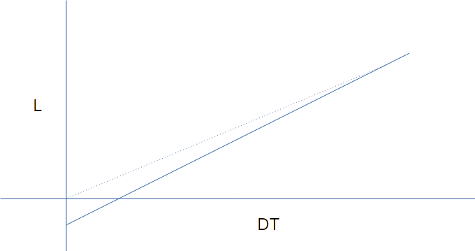
* Assuming you heat your house to 21, your DT intercept is at a negative DT instead of a positive one, suggesting probably a loss (or fixed consumption) somewhere in the system that does not end up in the fabric, or another artefact causing the same symptoms.  That was apparent earlier in your various plots and I have remarked upon it before, but its never been run to ground.

@cathoderay

Thank you for trying out the simple heat loss calculation that I suggested, the "HTC method". You have some excellent detailed data, which makes the analysis very interesting.

I noticed what appears to be a minor slip in your calculation. The heat from other sources was 320kWh over January, but then later this was 320W. These aren't consistent,  (320 x 1000)/(32 x 24) = 430W. HTC is still 493W/C, but the power from the heat pump is then 10.22kW.

@jamespa Your comment about HTC being the gradient of a line on the appropriate plot and the power from other sources being the intercept is spot on.

Both

The steady state equation balances the power going into the house with that coming out.

HSP + POS = HTC(IT - OT)

Where HSP is Heating System Power, OPS is Other Sources Power, HTC is the heating coefficient and IT and OT are indoor and outdoor temperatures.

Re-arranging, we have  HSP = HTC(IT - OT) - POS, which is the equation of a line of the form y = gx + c, where g (HTC in this case) is the gradient, and c is a constant equal to -POS in this case. So if we plot HSP vs. (IT-OT) on a graph as a lot of points and take a regression line, then the gradient should be HTC and the intercept on the y-axis (at a negative value) is POS.

While I was writing this @jamespa drew a nice graph of it!

An important point: the x co-ordinate needs to be the temperature difference (IT - OT) not just the outside temperature as on @cathoderay's graphs.

The key thing is that the equation is for the steady state equilibrium when the heat going in and the heat coming out of the house are equal. However, there is an issue with this. The outdoor temperature can change much faster than the indoor temperature. This is because the air outside has very little thermal inertia (heat capacity) compared to the house. This is easily observed on summer days when the heating is off. The swings in outdoor temperature between day and night can be very large, often 15 degrees or more, whereas a well-insulated house will only change in temperature by a few degrees. Further, there is a lag between the two cycles as the house take time to warm up and to cool down. Thermal inertia can be described in terms of a time constant, which technically is defined as the time for the temperature of an object move about 63% of the way towards thermal equilibrium with its environment, when that environment undergoes an instant change in temperature. This time constant can be quite long, e.g. a few days for a well-insulated house, more for one of stone construction.

This matters because it tells us something about the intervals of time that it would be appropriate to average over to get each data point for a graph. In this respect a day would be much better than an hour, and a few days better still, but then there may not be enough points. I would suggest using data for each day as a starting point as that at least averages out diurnal variations.

@cathoderay If you are willing, I would suggest grouping your January data by day. For each day, obtain the average power output for the heat pump, and the average values for indoor and outdoor temperatures, and hence the average for the difference in temperature. Then plot the 31 coordinates, one for each day, (x = average temperature difference for the day, y = average power from the heat pump for the day) on a graph and do the regression line for them. This should give a strong result for the gradient HTC and the power from other sources (minus value of y-axis intercept). It would also be interesting to see the same thing for the 744 hourly points. They will have much more scatter, but the regression should ultimately do a similar job to the daily averaging and I expect the results will be similar.

The graph that @cathoderay posted for January shows nearly all the points below the regression line where the outdoor temperature is below -2C. As noted this is because the heating is not quite enough in that case to keep the indoor temperature at the set point. This is distorting the results and likely pulling the calculated heat loss down. Plotting the data against temperature difference, which is the technically correct approach, rather than against outdoor temperature will sort this issue out.

OK, here is the IAT - OAT (degree-hours because the intervals are one hour) variant of the plot:

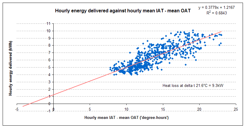
The intercepts show a different pattern: the intercept on the Y axis (@jamespa's L axis), which represents the fixed contribution from non-primary heat source sources is positive, which to me makes sense (they happen anyway, and so are always there, always positive, even in a heatwave), while the X axis (@jamespa's DT axis) intercept, the delta t at which the heating can be turned off, is negative, about -3°C, suggesting I can only turn the heating off when it is ~24°C outside, which is clearly not right. Something is wrong here! But I am not sure what it is.

Note the apparent left censorship (apparent removal of data on the left hand side) is because the month is January, and the delta T never dropped below around 6°C.   

@rob-of-york — I see you have just posted, I will post this, and then read and respond to your post  

Posted by: @rob-of-york

↑

I noticed what appears to be a minor slip in your calculation. The heat from other sources was 320kWh over January, but then later this was 320W. These aren't consistent,  (320 x 1000)/(32 x 24) = 430W. HTC is still 493W/C, but the power from the heat pump is then 10.22kW.

The 320 kWh total for all January was C29-C31 in your Practical Heat Loss Calculation spreadsheet, after I had entered my values in the relevant cells, and I understood it is the total for the whole month ie the 'x 31 x 24' has already been done. Thus the total energy delivered over the month = 4612 kWh from the heat pump + 320 kWh from other sources = 4392 kWh in total which I then divided by 10005 degree-hours to get a HTC of 0.493 kWh/C or 493W/C. However, as you say (I'm spelling this out to (a) confirm I have got it right and (b) perhaps helps other trying to understand all this), I then used a figure of 0.32 kW (kW rather than W because the heat loss is in kW) which was simply my total other heat source energy (320 kWh) divided by 1000 for reasons I cannot explain (perhaps calculation fatigue). The correct figure is as you say the monthly total converted to an hourly rate, because behind the scenes the heat loss is the hourly rate, and so it should be (in kWh) 320 / (31 [sic] x 24) = 0.430 kW, or 430W.

Posted by: @rob-of-york

↑

So if we plot HSP vs. (IT-OT) on a graph as a lot of points and take a regression line, then the gradient should be HTC and the intercept on the y-axis (at a negative value) is POS.

While I was writing this @jamespa drew a nice graph of it!

And I then posted my real world data plot, where the Y axis intercept is positive rather than negative! I think I can see, by my weird logic, that, because the line is solely the heat pump energy, it should be negative, because it is the energy the heat pump does not need to provide, because it is provided by the other sources, if that makes sense. Yet in my plot it is positive...which needs to be resolved.

The discussion about what interval to use is interesting, and makes sense. I have already posted the 744 hourly points using IAT - OAT, and can do the same for daily averages. Bur before I do so, I just want to be sure it is hourly averages of the energy delivered, not the sum (total) for the day? Is it because by convention the heat loss is based on an hour, ie it is the power a heat pump needs to run at for an hour (which is why the heat loss, quoted as power in kW, is also the energy over one hour, in kWh) to maintain the IAT?     

Posted by: @rob-of-york

↑

The graph that @cathoderay posted for January shows nearly all the points below the regression line where the outdoor temperature is below -2C. As noted this is because the heating is not quite enough in that case to keep the indoor temperature at the set point. This is distorting the results and likely pulling the calculated heat loss down. Plotting the data against temperature difference, which is the technically correct approach, rather than against outdoor temperature will sort this issue out.

This makes sense, and the plot of energy against IAT - OAT rather than just OAT does appear to sort this out (even dispersion across the range of IAT - OAT, might be worth doing some residual and other diagnostic plots) in my later plot. But interestingly both plots suggest the same heat loss, 9.3 kW, maybe because it is the same data? Another option might be to remove the very low points (say sub zero OAT, because at those OAT's the heat pump can't quite cope)  so they don't pull the regression line down at the lower OAT end.

Posted by: @cathoderay

↑

The intercepts show a different pattern: the intercept on the Y axis (@jamespa's L axis), which represents the fixed contribution from non-primary heat source sources is positive, which to me makes sense (they happen anyway, and so are always there, always positive, even in a heatwave),

It may make sense but its not as expected, it should be negative.  You are plotting delivered energy to the house vs DT and if there is a positive contribution for other sources the intercept on the Y axis should be negative.  

Posted by: @cathoderay

↑

while the X axis (@jamespa's DT axis) intercept, the delta t at which the heating can be turned off, is negative, about -3°C, suggesting I can only turn the heating off when it is ~24°C outside, which is clearly not right. Something is wrong here! But I am not sure what it is.

consistent with the above.

Posted by: @cathoderay

↑

Something is wrong here! But I am not sure what it is.

Correct, there always has been something wrong, I have observed that about your system for some while and mentioned it a couple of times.  You appear to have a fixed loss (ie when DT=0 you still have to supply the house with energy to keep it at a constant temperature) not a fixed gain.  Since you for certain do have a fixed gain the fixed loss is apparently quite high, high enough to overcome the gain then some.

I think you would have a better chance of working out what it is if you had some more data closer to the origin.  You have several times commented on the risks of excessive extrapolation, and here you have excessive extrapolation if the task is to identify the cause of the apparent