@jamespa and @rob-of-york — thank you both very much I think I have now got it well enough to retain it! The light bulb paragraph for me (I am better at abstract conceptual thought using words rather than maths) is this one

:

Posted by: @rob-of-york

↑

What do the new data points look like on the graph? Answer, exactly the same as the old data points, but the scale on the y-axis has shifted by 1kW. (Note this assumes that none of our original data points required less than 1kW from the primary heating system). The regression line now hits the y-axis at -1kW. The primary heating system puts out 1kW less at any given time relative to the situation without the additional source of heat. However, nothing here changes the slope of the graph. If the temperature difference increases by 1C, then it is the primary heating system that has to provide the extra power equal to HTC. The additional source of heat does nothing different, it just sits there delivering 1kW. 

In particular "but the scale on the y-axis has shifted by 1kW" (even if perhaps it is the regression line that shifts, not the scale on the y-axis, is the line drops rather than the axis scale rises) and then "However, nothing here changes the slope of the graph", ie the HTC remains constant, whatever the value of PO.

I even managed to sail past this point without noticing its importance in my chart with the second dotted line! When I added the line, I was careful to make it parallel, ie not change the gradient, somehow appreciating, but not understanding, that HTC, the gradient, stays the same.

At this point its probably worth pointing out, for future reference, that degree days are not exactly the same as an offset average OAT. 

There is an explanation here, but in essence degree days count the time that the OAT is below the base temperature * the number of degrees it is below and completely ignore any time that the OAT is above the base temperature.  So for example if the outside temperature is 10.5 for half a day and 20.5 for half a day (a pattern which can happen in spring!) the number of degree days is 0.5*5=2.5 which you might (erroneously) equate to an average OAT of 15.5-2.5=13, whereas the actual average OAT is 10.5*.5+20.5*5 =15.5.  

This really only matters at the beginning of Autumn and the end of Spring, so for most practical purposes can be ignored.  Nevertheless its worth keeping the difference in the back of your mind if you are doing calculations based solely on data from early Autumn or late Spring which, TBH, I would not recommend as they inevitably involve far too much extrapolation.

Re

Posted by: @rob-of-york

↑

A refinement of the degree-day method

The degree day method of heat loss calculation is very useful because it only requires smart meter data on daily gas usage, which nearly everyone can obtain, and Met Office degree day data from a nearby weather station, which is again readily available.

The downside is that it is less accurate than using the difference between indoor and outdoor temperatures measured by a home weather station.

The question is what can be done to refine the degree day method to obtain better accuracy, without needing a lot more data. This post attempts to answer that question.

 

I think your proposed refinement where the house is heated part time is reasonable.  There are a couple of things to observe:

• The correction factor (0.95) that you have calculated illustrates quite nicely that the very optimistic savings (20-30%) that some people (and some manufacturers of controls) claim from part time heating are just that!
• This is one of a few correction  factors which are probably around 5-10% and may or may not apply depending on the starting data.  The others including
  • Boiler 'efficiency'* (75%-110%, but usually 90-95%)
  • DHW load (depending on whether you include it)
  • Extraneous losses eg if the boiler is in an unheated space like a garage
  • Wind factors
  • Solar gain over the season
  • partial heating of the house (spatially)
• It would be interesting at some point to develop a list and estimates for all of them.  However I suspect that the outturn result will be 'dont bother' (with the corrections) unless you are really borderline between two heat pump models; the answer is good to about 15%, get over it, that's stlll way better than any survey!

Posted by: @jamespa 

At this point its probably worth pointing out, for future reference, that degree days are not exactly the same as an offset average OAT. 

Thanks for pointing out that nuance, I had not picked up on it. The data that I am using for Oct to March has no days with an average daily temperature over 15.5, the smallest Degree Day is 1.2, with no negative values. However, I suspect that if I were to look at Degree Hours instead, some of them may have outdoor temperatures over 15.5C.

One thing I find slightly questionable about these measures that comes about because of the MAX, e.g. DH = MAX(0, 15.5 - OTh) for degree hours. They don't have a sort of scale invariance property. Quantities such as average, min, and max temperature have this invariance in the sense that your can work out the average over a day from the averages for the hours in that day, which in turn can be worked out from the averages for each minute in the hour. With Degree Days, Degree Hours, and Degree Minutes (if there is such a thing) they don't have that relationship because of the MAX limiting to no less than zero.

The correction factor (0.95) that you have calculated illustrates quite nicely that the very optimistic savings (20-30%) that some people (and some manufacturers of controls) claim from part time heating are just that!

Nice interpretation. By not heating overnight, the daily average indoor temperature drops by just 5% and the overall heating demand by about the same. Not a huge difference, and the cost saving is perhaps smaller still if the heating is less efficient when it has to work hard to raise the temperature of the house back to the set point. 

• This is one of a few correction  factors which are probably around 5-10% and may or may not apply depending on the starting data.  The others including

  • Boiler 'efficiency'* (75%-110%, but usually 90-95%)
  • DHW load (depending on whether you include it)
  • Extraneous losses eg if the boiler is in an unheated space like a garage
  • Wind factors
  • Solar gain over the season
  • partial heating of the house (spatially)

• It would be interesting at some point to develop a list and estimates for all of them. 

That's a good point. I'm going to go back to my heat loss calculations based on temperature differences, with gas and electricity consumption included, i.e. the best data that I have and think through the impacts of these factors and any others that I can think off. The idea being to ensure that any unaccounted for effects (e.g. solar gain) or errors in estimates (e.g. boiler efficiency) lead to an overestimate in the heat loss calculated or a range of values for heat loss that can be quantified. 

Posted by @jamespa

It would be interesting at some point to develop a list and estimates for all of them. 

Below I've considered the impact of the following on the graphical method of HTC and heat lost estimation based on measured data:

1. Accuracy of the input data: How accurate the temperature and energy usage data are that the calculation is based on.
2. Energy conversion efficiency: How much of the energy from each unit of gas ends up as useful heat in the house.
3. Additional heating: Other factors that can add heat to the house.
4. Additional losses: Other factors that can result in additional heat loss.

The various factors are marked as either (i) Inconsequential – if the uncertainty is so small as to be inconsequential, (ii) Pessimistic – if the uncertainty leads to an overestimate of the heat loss, (iii) Optimistic – if the uncertainty may lead to an underestimate of the heat loss, which should be avoided, and (iv) Ignored – if the factor discussed has no impact on the HTC value obtained and hence the heat loss.

1. Accuracy of input data

The number of units of gas and electricity used are highly accurate, since these numbers are used for billing. (Inconsequential)

The outdoor temperature reading is accurate to +/-0.1C for the location in the back garden where the weather station is located. Variation with respect to where the house is less than 10m away is likely to be small. (Inconsequential)

The indoor temperature sensor is in the living room. This room is typically slightly cooler than the average for the upstairs rooms, since heat rises through the house. It is typically slightly warmer than the hallway, kitchen and utility. The temperature recorded in the living room is likely close to the average for the house. (Inconsequential)

Conclusion: The raw input data is sufficiently accurate to be used in the graphical HTC and heat loss calculations.

2. Energy conversion efficiency

There are a number of factors at play here. A gas boiler is used for heating and hot water. It is sited in an unheated space and uses weather compensation.

Assuming a higher overall efficiency than is actually achieved is pessimistic, since it results in a higher number for the power going into useful heating, hence any boiler efficiency estimate should err slightly on that side.

Note, boiler efficiency has a theoretical maximum of 100% compared to the gross calorific value (or kWh) of the units supplied e.g. as shown on a gas bill.

For space heating, the boiler runs a weather compensation curve. At the time (Oct’24 to Mar’25) this was set to 67C flow at -5C outside temperature, 61C at 0C, 54C at 5C, 46C at 10C. Assuming that the return was 20C lower in temperature this gives return temperatures of 47C, 41C, 34C, and 26C.

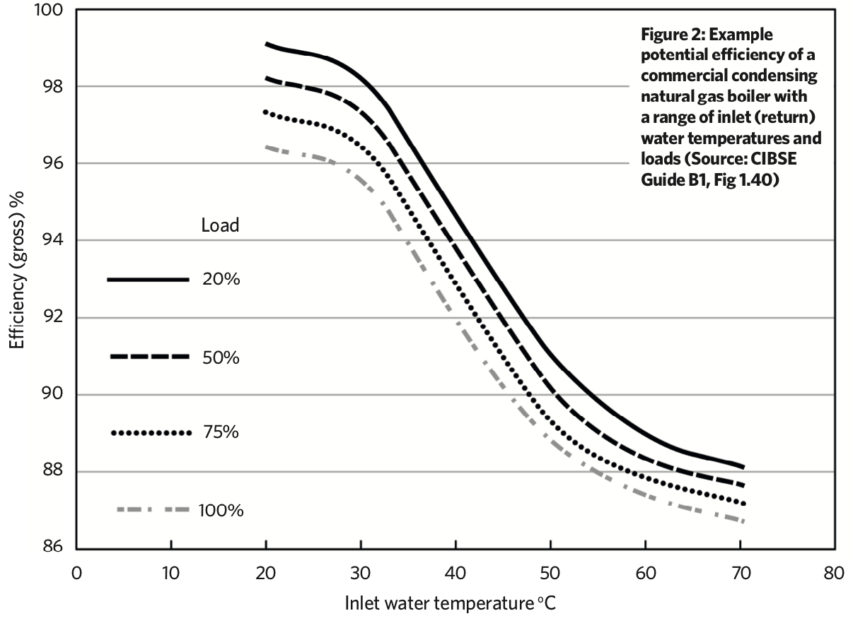
Boiler efficiency values were taken from the above graph by looking up the flow temperature from the weather compensation curve based on the average daily outdoor temperature. DT20 was assumed, i.e. return temperature 20C lower than flow. It is unlikely that the temperature difference was this high, however this assumption ensures that the daily boiler efficiency values remain optimistic and hence the heat output to the house is not underestimated. The efficiencies used were taken from the 50% load line, since the boiler has a capacity of 24kW and the radiators only 12kW.

When heating hot water, the flow temperature is 80C and the return about 60C for an efficiency of 88%. As hot water heating is a relatively small fraction of the total, this difference in efficiency was not accounted for. In other words, the efficiency for space heating was assumed for all of the gas usage. This is a pessimistic assumption with respect to the heat loss calculation, since the achieved efficiency would be slightly lower.

The gas boiler is in an unheated space. Heat is lost to that space by the boiler, and this is estimated to result in a 2% reduction in boiler efficiency.

Conclusion: Daily boiler efficiency values are used based on the outdoor temperatures and the weather compensation curve. Efficiency is reduced by 2% due to the boiler being sited in an unheated space. The lower efficiency of hot water heating is not accounted for resulting in a small overestimate of the heat loss.

3. Additional heating

The consistent presence of people in the house provides a constant low level of power output (about 100W each), since this is effectively constant, it does not affect the slope of the regression line and so is Inconsequential.

Solar gain can be estimated by considering window glass area, orientation, and the g-value for the glazing. For my house, the incident energy on the windows was assessed using PVWatts modelling of the window orientations (vertical, NSEW) and their area. Overall solar gain works out at 67% of the output of my Solar PV system over the Oct to March period.

Solar gain was accounted for as 0.67 of the Solar PV production for each day.

Conclusion: Solar gain is accounted for using a percentage of the solar PV output with the percentage calculated based on window areas and orientation. The consistent heating effect of people in the house was not accounted for as it does not affect the HTC calculation.

4. Additional losses

One form of additional loss comes from hot water that vanishes down the drain along with the heat that it carries. Including the power needed to heat hot water is a pessimistic assumption, since a significant fraction of this power does not contribute to heating the house, only the losses through the very heavily insulated hot water tank. The heat loss via hot water draining away is not part of the fabric heat loss of the house.

Weather conditions that were not seen over the time period in which the data was collected. For example, high winds that cause more heat to be lost by the building than seen in the observed data. Since the data was not representative of these conditions, then the HTC value and heat loss calculated may be optimistic for this case. There is no easy way around this, other than adding some guessed at margin for error, or accepting that in some circumstances, including outdoor temperatures below the design temperature, supplementary heating may be required. My preference is the latter.

Conclusions: Including the power for hot water heating in the input data is a pessimistic assumption. Either a margin for error needs to be added to account for rare weather conditions not seen during the observation period, such as high winds and very low temperatures, or accept that this situation can be covered by supplementary heating.

5. Heat loss and heat pump sizing

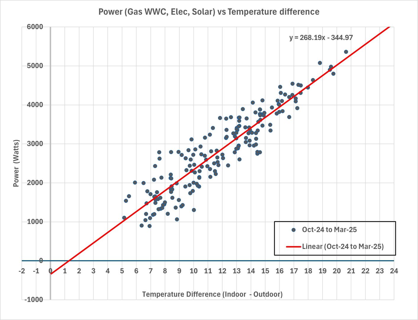
Considering variable gas boiler efficiency due to weather compensation, and additional heat from daily electricity use, and daily solar gains, the total heat loss at 24C temperature difference is estimated at 6440W or 6260W if 180W for hot water heating are excluded.

Using the higher heat loss figure for heat pump sizing would be sufficient to cover the following worst-case situation. Outside temperature -3C, indoor temperature 21C, no heat from any other sources (solar gain, electricity use, and people). It is also enough to cover the hot water heating.

In practice, 290W is on average provided by background electricity use and around 130W by two people present 16 hours per day. This leaves 6020W to be provided by a heat pump to satisfy space heating and hot water requirements, hence a 6kW heat pump would suffice.

It is interesting that including more detail in the power output figures (e.g. variability in boiler efficiency due to weather compensation, daily electricity consumption, daily solar gains) made very little difference in the HTC value and hence the heat loss estimate. This is likely because the variability in these factors is relatively small compared to the differences between heat loss on cold versus warm days, and the variability tends to average out over the 6 month period.

Conclusions

I think I've now got the heat loss calculation via measurements as accurate as I reasonably can. The overall heat loss calculated by various methods (including a detailed theoretical model) is in the range 6.0kW to 6.5kW. With at most 6kW needed to be supplied by the heating system. Further, if extreme weather conditions below the design temperature mean that a 6kW ASHP cannot quite keep up that would be no problem, since the air-to-air system (2.5kW and 3.5kW) can easily provide the extra required.

Posted by: @rob-of-york

↑

Note, boiler efficiency has a theoretical maximum of 100% compared to the gross calorific value (or kWh) of the units supplied e.g. as shown on a gas bill.

 

I have seen it stated that the declared calorific value does not include latent heat of condensation (which is very plausible) and therefore that, in principle, a well adjusted condensing boiler could supply >100% of the metered amount.  I have not seen experimental evidence to support the latter part of the sentence and, given that most gas boilers are grossly over sized and run at a FT that is way too high, I suspect this rarely if ever occurs

Posted by: @rob-of-york

↑

It is interesting that including more detail in the power output figures (e.g. variability in boiler efficiency due to weather compensation, daily electricity consumption, daily solar gains) made very little difference in the HTC value and hence the heat loss estimate. This is likely because the variability in these factors is relatively small compared to the differences between heat loss on cold versus warm days, and the variability tends to average out over the 6 month period.

Conclusions

I think I've now got the heat loss calculation via measurements as accurate as I reasonably can. The overall heat loss calculated by various methods (including a detailed theoretical model) is in the range 6.0kW to 6.5kW. With at most 6kW needed to be supplied by the heating system. Further, if extreme weather conditions below the design temperature mean that a 6kW ASHP cannot quite keep up that would be no problem, since the air-to-air system (2.5kW and 3.5kW) can easily provide the extra required.

Great stuff!