@cathoderay I see you are continuing to misquote from the thread below.

https://renewableheatinghub.co.uk/forums/postid/28542

What you are repeatedly failing to see is that my thread is about making a simple symmetrical comparison between energy used for several days at different OATs. The control is a target comfort temperature for a specified daytime period.

the trials were done using only the Mitsubishi generated data with no elaborate data gathering. Since I’m a firm believer that -

Information is not Knowledge  

Furthermore I have been mindful of the mixed level of understanding of the audience of these topics. And therefore of the need to keep a degree of succinct messaging. If you don’t like that then that’s fare enough you don’t have to read them. However you have chosen to mis quote and cast doubt indiscriminately on the outcome of someone else’s work.

in your replies you misquotes the number of 24/7 trials I had done for example.

you have repeatedly said there were no controls on comfort room temperatures when clearly there were.

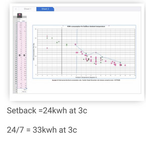
here was the last scatter graph showing the last 24 hour consumption that you appear to have failed to have seen.

In this last 24 hour, operated HP period it was on a cold night and was below 3c getting colder. It was fully within our defrost temperature zone. This meant the HP operated through repeated defrost cycles. The results were unequivocal. The HP  used 9 kWh more energy during continuous night time operation than the several nights of the same OAT using the setback operation. 

The savings were especially high during sub 3c ambients. And since I was funding this trial then I felt my trial had run it’s course.

So in the space of 3 months (and only 3 pages of the topic thread) the trials had established clear trends of higher energy usage.

By comparison I note that your earlier thread “Do setbacks save energy without compromising comfort” it ran for 71 pages and 843 posts. It’s what prompted me to do a simpler study.

In the end we are homeowners helping each other out. Or at least that’s why I joined this forum.

@sunandair I don't want to get embroiled in an argument, but I am interested in finding a tolerably robust answer to the question that can be applied to multiple systems because, as you say, this forum is about homeowners helping each other out. 

Unless we understand and can explain the results from any individual system/set of circumstances (whatever they show), we have no idea how, or whether, it will apply to any other.  For me the understanding of experimental results is thus as important as the experimental results themselves.  The exception to this would be if we had a fairly large number of results from multiple systems in multiple circumstances.  Sadly, we don't and its unlikely we will.  

I have asked twice whether you would be prepared to share the data and explain what the annotations mean, but you haven't replied.  At the risk of antagonising you I will ask a third time, but this will be the last. 

My objective in making this request was to be able to do a bit of analysis to see what I might be able to explain using basic physics.  Alternatively perhaps you might be willing to do this yourself?

Without an plausible explanation of the observed phenomena (that as a minimum accounts for conservation of energy) I am not confident to draw conclusions from your system that are applicable to any system other than yours, and will be therefore sticking with my current position (which amounts to: we don't know for certain - in some circumstances, probably, in others, probably not).  You are of course at liberty to do something different.

Posted by: @sunandair

↑

In the end we are homeowners helping each other out. Or at least that’s why I joined this forum.

We certainly are, and that's why I am here too. But that doesn't mean we shouldn't have have robust discussions. Indeed one of the remarkable things about this forum, and I think has a lot to do with the way @editor runs things, is that is is both remarkably civil and yet capable of sustaining robust discussion at the same time.

I haven't dismissed your findings and I applaud the idea of simple messages but one thing I have learnt about the setback question is that it is an extremely challenging one to answer. Indeed that is the reason why the previous setback thread clocked up so many pages and posts - there isn't a simple general answer yet.

I stick by my assertion that you have only posted limited data, particularly on comfort (IAT). Strictly speaking the control isn't a "target comfort temperature for a specified daytime period", what we are doing to do is control for IAT, ie make sure we are comparing like with like. As I said, I think you have only posted two charts showing IAT behaviour over two 24h periods (and no numerical data) and (a) they are equivocal and (b) they are simply not enough data. I think, if I have read your posts right, you have only had a total of four 24h periods of continuous running, and that is an extremely small sample size.

The problem we have is we can't do controlled experiments (two identical houses in two identical environments, one running a setback, the other not running a setback) so we have to do so called natural or observational experiments but in reality these are studies, not experiments, even if we do change one the parameters (heating pattern). To stand any chance of making sense of the observations, we have to record other variables and somehow adjust for them, there being a number of standard ways of doing this, with stratification (dividing into bands) being the classic approach. Thus we might compare cold days with setbacks with cold days without a setback, and warm days with setback with warm days without setback, the stratification here being by OAT. Having only four no setback days is just too small a sample.

@jamespa has very sensibly asked if you have any numerical data in a usable format that you can post. Data sharing used to be the norm in science (its all part of the replication process), and indeed, failure to publish raw data is a bit of a red flag in my book (and there are certain very well known examples). Sketchy or obfuscated methodology is another red flag. All these unfortunate habits tend to get in the way of getting the right answers.

I am also concerned, assuming I have read your posts right, about your way of recording the OAT for a 24 hour period. If it is 'min value plus one third of the range' for the 24h period, then I don't think it is a viable way of recording the 'overall' picture of the OAT over a 24h period. Given the general noise, and number of other variables in play such biases (systematic errors that that distort results away from the correct result, in contrast to random errors) could seriously weaken the validity of any conclusions.

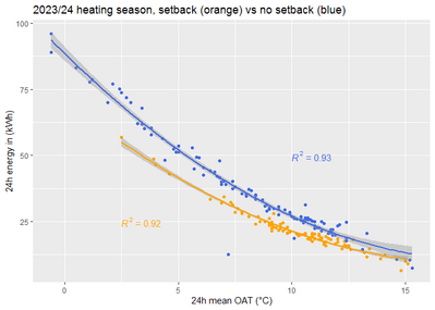
Meanwhile I have managed to make some progress on the question of whether my setback data and non-setback data (with hundreds of observation in all) are samples from the same population of not - in simple terms, are they different suggesting there is a difference when using a setback, or is the visual difference, which is certainly there, just down to random variation. Although this is in fact a simple null hypothesis question (testing the hypothesis that there is no difference), I haven't been able to find a satisfactory (to me) single numerical statistical test for this, but I have done a plot (in R for those who want to know) of the two samples and added a polynomial (2nd order) regression line, which provides a very good fit, with the 95% confidence intervals (grey shaded zone around each line). As these are visually separate (apart from the extreme right hand end, where there is virtually no data), is is highly unlikely they come from the same population, or to put it in plain English, something different does appear to happen with setback running.

I am not yet ready to say this is a definitive answer, but it is certainly pointing that way (the two samples are from different populations). I have another test I want to try, and also, if I can, replicate the above in python.

I see @jamespa has posted while I was writing this, some perhaps inevitable overlap.

And here in case any one wants it is the code I used in R:

#read the data, already has grouping variable setback, 1 = with setback, 0 = no setback 
df_htg <- read.csv("D:\\Monitoring\\24h avg amb vs htg kWh in 23-24 season.csv")

# split dataframe into two, one for setback values, one for no setback values
df_sb <- df_htg[df_htg$setback == 1, ]
df_nosb <- df_htg[df_htg$setback == 0, ]

#load necessary libraries
library(ggplot2)
library(ggpubr)

#do the plot
ggplot() +
  geom_point(aes(x=amb_24h_mean, y=htg_24h_kWh_in), data = df_sb, color = "orange") + 
  geom_point(aes(x=amb_24h_mean, y=htg_24h_kWh_in), data = df_nosb, color = "royalblue") +
  stat_smooth(aes(x=amb_24h_mean, y=htg_24h_kWh_in), data = df_sb, 
              method = "lm", formula = y ~ x + I(x^2), color = "orange") + 
  stat_smooth(aes(x=amb_24h_mean, y=htg_24h_kWh_in), data = df_nosb, 
              method = "lm", formula = y ~ x + I(x^2), color = "royalblue") +
  labs(title="2023/24 heating season, setback (orange) vs no setback (blue)", x="24h mean OAT (°C)", y="24h energy in (kWh)") +
  stat_cor(aes(x=amb_24h_mean, y=htg_24h_kWh_in, label = paste(..rr.label..)), data = df_sb, label.x = 2.5, label.y = 25, color = "orange") +
  stat_cor(aes(x=amb_24h_mean, y=htg_24h_kWh_in, label = paste(..rr.label..)), data = df_nosb, label.x = 10, label.y = 50, color = "royalblue")
  

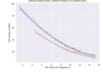
Here's the same plot, less the R squared values, done quick and dirty in python, with the one done in R on the right:

They look the same to me apart from the extreme left hand end of the setback confidence interval, an artefact most likely due to the small number of samples in that region.

Different method, same result, confidence grows.

Python code for anyone who wants it:

import numpy as np
import pandas as pd
import seaborn as sns
import matplotlib.pyplot as plt

sns.set_theme()

df = pd.read_csv(r'D:\DIY Monitoring\24h avg amb vs htg kWh in 23-24 season for R.csv', 
      skiprows=1, usecols=[1,2,3], names=['amb','kWh','sb'])

g = sns.lmplot(data=df, x="amb", y="kWh", hue="sb",
      order=2, ci=95, legend=False, scatter_kws={"s": 4})

g.set(xlabel ="24h mean OAT (degrees C)",
      ylabel = "24h energy in (kWh)",
      title ="2023/24 heating season, setback (orange) vs no setback (blue)")

plt.show()

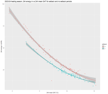
And finally, the R version tidied up a bit and larger, so 95% confidence interval bands are more visible:

The R code used (slightly different, but in essence does the same thing):

# read the data, already has grouping variable setback, y = with setback, n = no setback 
df_htg <- read.csv("D:\\24h avg amb vs htg kWh in 23-24 season for R.csv")

#load necessary libray
library(ggplot2)

#do the plot
p <- ggplot(data = df_htg, aes(x = amb_24h_mean, y = htg_24h_kWh_in, color = setback)) + 
  # add data points
  geom_point() +
  # add 2nd order polynomial regression with 95% confidence intervals
  stat_smooth(method ="lm", formula = y ~ x + I(x^2)) +
  # add titles
  labs(title="2023/24 heating season, 24h energy in vs 24h mean OAT for setback and no setback periods", 
     x="24h mean OAT (°C)", y="24h energy in (kWh)")
print(p)

For completeness sake, and I may as well document it here as anywhere else, I have now done the other test I mentioned earlier for whether the two samples, with setback and without setback, appear to come from the same populations or not, the inference being that if they come from different populations, then that suggests there is a real difference between energy use in setback running vs non-setback running. 

The test is entirely different to the previous ones, and is based on a simple idea: first run a regression on the whole data set (setback and non-setback all together) and the repeat the regression, this time adding setback/no setback as a grouping variable, which has the effect of adjusting for the presence or absence of setback running. The idea is that if adding the setback/no setback variable improves the fit and the two are statistically different - in other words, incorporating the setback variable makes a demonstrable difference - then the two groups are different. The idea comes from this thread on Cross Validated. I appreciate this is getting into rather academic territory, and may even be getting close to my black box statistics variation of Dennis Healey's First Law of Holes, when doing black box statistics (no idea what is going on inside), stop doing them, but I record it here, as I say, for completeness. Any comments are of course very welcome. The code and results are as follows:

#read the data, already has grouping variable setback, y = with setback, n = no setback
df_htg <- read.csv("D:\\Monitoring\\24h avg amb vs htg kWh in 23-24 season for R.csv")

# do the regression first without , and then with, the grouping variable
fit0 <- lm(htg_24h_kWh_in ~ amb_24h_mean + I(amb_24h_mean^2), data = df_htg)
fit1 <- lm(htg_24h_kWh_in ~ amb_24h_mean + I(amb_24h_mean^2) * setback, data = df_htg)

#compare the two
anova(fit0,fit1)

**Results**

Analysis of Variance Table

Model 1: htg_24h_kWh_in ~ amb_24h_mean + I(amb_24h_mean^2)
Model 2: htg_24h_kWh_in ~ amb_24h_mean + I(amb_24h_mean^2) * setback
Res.Df RSS Df Sum of Sq F Pr(>F)
1 196 3446.5
2 194 1622.7 2 1823.8 109.03 < 2.2e-16 

What the above results (claim to) tell us is that:

(a) model 2 (the one with the setback grouping variable) is the better fit to the data (shown by the lower RSS or residual sum of the squares value)

(b) the difference between the models is statistically significant (shown by the very low Pr(>F) value, which here acts like a normal p value).

In other words this completely different test gives us the same conclusion: the setback sample and the non setback sample come from different populations, the relationship between 24 hour mean OAT and 24 energy use when running with a setback is not the same as running without a setback, something is different.

Edit: code moved out of code block as WP CSS rendered the code FUBAR and I can't be bothered to nuke the pesky WP CSS 

Edit2: still messed up, but less so...     

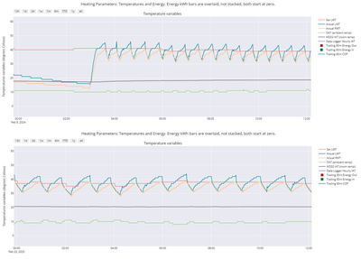
@cathoderay Whilst trying to do an energy analysis I looked a bit more closely at the  two plots you posted of similar days.  The cycling, once you are past the bulk of the recovery period in the setback case) is starkly different between the two, even though the conditions and target FT are very similar.

For example compare 6 hours starting 06:00 Feb 9 2024 with 6 hours starting 06:00 Feb 23 2025.  In the first of these there are 11 cycles.  In the second there are only 6 cycles.  The peaks and troughs are essentially the same in both cases, but the behaviour is very different.

I dont see any reason to think this is due to setback, I think its more likely due to the changes you made in your system.  Its a big (and I think positive) difference though!

Regarding the energy balance calculations (first stage - attempt to reconcile the difference between 'energy out' in the setback and the non setback with conservation of energy), I'm not really making much progress.  The problem is the heat capacity of the house has the potential to dominate the calculation, even though the changes in house and ambient temperature during both setback and non setback periods are small.  However this is a massive unknown - whilst we can be fairly certain that your house heat capacity is order 10-15kWh/C, we really have little clue about the dynamics of this.  It will take time, possibly more than 24 hr, for the fabric to 'readjust' to OAT and IAT changes (a emphasised because of course this is what we measure), ao its difficult to tell the extent to which these will 'feed through' to the energy balance in the period or whether, for example, I should be looking at what happened 24-48 hours previously.  The advantage of measurements over longer periods is that the heat capacity component becomes a smaller proportion of the calculation, but the probability of nature cooperating to provide such periods shrinks, I suspect exponentially.  I've still got a few more angles on the calculation though, so maybe that will bear fruit.

@jamespa - thank you for your ongoing heroic attempts to make sense of all this.

Posted by: @jamespa

↑

For example compare 6 hours starting 06:00 Feb 9 2024 with 6 hours starting 06:00 Feb 23 2025.  In the first of these there are 11 cycles.  In the second there are only 6 cycles.  The peaks and troughs are essentially the same in both cases, but the behaviour is very different.

I dont see any reason to think this is due to setback, I think its more likely due to the changes you made in your system.  Its a big (and I think positive) difference though!

I too had noticed this different behaviour. Here are the two periods next to each other for comparison:

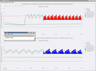
There are a number of possible variations that occur to me. Firstly, the upper 2024 plot has a setback, the lower 2025 doesn't. As a consequence, the IAT is lower in the upper 2024 plot, and it may just have been low enough to trigger a small LWT boost from my auto-adapt script. Secondly, although the OATs are similar, other weather factors, including both wind speed and direction and exposure to sunlight (the heat pump is on an east facing wall) may have come into play. And of course as you say the second period is after 'big bang', the day when I opened up all the lock shield valves to get a truly open system. It might be interesting to look at areas under the curves, to see if they are different, but not easy to do. I could try filling the spaces with a unique colour and then counting the pixels... 

Flood fill and colour count reduction done in Photoline, pixel count per colour done in ImageJ. The Log window shows the RGB fc0000 red pixel count, 25,434. The number for 0000fc RGB blue is 22,960. An online pixel colour counter gives the same results. Given the constraints of the methodology, these areas are similar if not effectively the same. 

With his permission I did some analysis on the plots of 'similar days' posted by @cathoderay a few posts ago. 

The most important thing that comes out is that 'eyeball integration'  is not reliable - the post suggested (based on an 'eyeball integration' that certainly convinced me) that there was a substantial difference (~5kWh) between the energy supplied to the heat pump (ie electricity use) in the setback case, vs the non setback case.  However when you look at the actual data and add up the figures, the difference is, in fact, very small (<1kWh - 4%).  Interestingly the difference in energy supplied by the heat pump (ie heat to house) is large (29kWh, =27%).  

The saving in electricity consumption is actually quite close to what my simulations of setback would predict for the parameters in question, but I cant account for the energy balance in the heat to the house and, until we can, its very difficult to have any level of confidence at all that we understand whats going on.

The heat pump in both samples cycle, and its noticeable that the cycle frequency in the 'setback' sample is about twice that in the 'continuous' sample.  I think the most likely explanation for this is changes to the system made by OP between the two measurements, but this is speculation.  I cant see that this obviously explains the big difference in energy supplied by the heat pump. 

Comments or enlightenment welcome - although I fear this may be yet another illustration of how difficult it is to get to a sound conclusion that is applicable to any system other than the one it was measured on!

@jamespa sounds like it should be a job for Octopus to test in their controlled conditions  so they can test different scenarios!

https://octopus.energy/blog/energy-house-2/

Posted by: @tim441

↑

@jamespa sounds like it should be a job for Octopus to test in their controlled conditions  so they can test different scenarios!

Definitely - I didnt realise that they had a stake in the house in warehouse.

Octopus also have access to 'big data' from their installed heat pumps and their energy metering.  So they are in a position to analyse this also, which I have an idea may well suffice to give tolerably reliable general guidance.