@cathoderay I would suggest you investigate the power requirements of your circulating pumps and subtract that figure from your daily energy in calcs in order to get a clearer picture. If a pump is using say typ. 50 watts and you have two of them running then that would equate to 2.4kWhr per day and would show your system needing this energy input even when the OAT was 20degC. (and IAT of 19!) surely?

On the 9 Dec your energy in was 26.91kWhr..perhaps10% of this could be attributed to the circulating pumps?

It's also 2.4kWh extra heat generated in your home (assuming the circulating pumps are inside the thermal envelope of your home).

Posted by: @iaack

↑

@cathoderay I would suggest you investigate the power requirements of your circulating pumps and subtract that figure from your daily energy in calcs in order to get a clearer picture. If a pump is using say typ. 50 watts and you have two of them running then that would equate to 2.4kWhr per day and would show your system needing this energy input even when the OAT was 20degC. (and IAT of 19!) surely?

On the 9 Dec your energy in was 26.91kWhr..perhaps10% of this could be attributed to the circulating pumps?

Posted by: @scrchngwsl

↑

It's also 2.4kWh extra heat generated in your home (assuming the circulating pumps are inside the thermal envelope of your home).

I do agree, how the the circulating pumps are treated for energy use is an unknown. I've been inclined to suppose they were part, maybe most, of the explanation for the 1.18 discrepancy factor between the calculated energy in and the metered energy in. We don't know how of where Midea measures amps in, which is the major determinant of energy in, given volts in are reasonably stable. Somewhere I think I saw something that suggested it was compressor amps, but I can't find that reference again, and I think it is very plausible it doesn't include the external secondary circulating pump, which often won't be present. This pump is inside the thermal envelope of the house, and so it won't all be lost heat, the primary circulating pump is in the outside box, and any heat from it will be lost.

Posted by: @jamespa

↑

I would have reached the same conclusion except that the scattergram of corrected IAT-OAT vs energy out (corrected for the thermal mass of the fabric), which I previously posted, has a similar intercept.  This is also the scattergram which shows the best correlation of all of the correlated data points - a fact that's rather encouraging because its the one that has the most solid underpinning in physics.  So I am pretty convinced that the intercept is real.  As to how it should be interpreted, well that's another matter!

We need to know more about the PHE.  Can you tell us anything about temperature differences between the ports?  Also, I'm wondering what the quiescent consumption of the heat pump is, and whether its included in the figures that come out of it (something, after all, is accounting for a factor of 1.18).

There has to be something which explains why you can get away with (apparently) dumping 20% less energy into the house for a few days and it only cools on average by a fraction of a degree.  So far we don't have a plausible explanation so we need to keep looking.  Otherwise any conclusion we might attempt to reach from the experimental results applies only to your specific system in the specific conditions of the experiment, which is not a lot of use to anyone other than you.

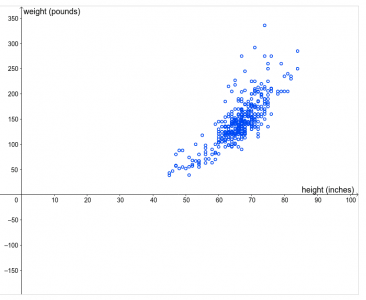
I wonder if we might be making one of the oldest mistakes in the book, extrapolating beyond observed data. For example, here is a random height vs weight plot I found online. Even without adding a trend line, we can see something will go wrong if we do add one, and extend it. At a height of about 40", the creature vanishes (perhaps a vampire got them?) as they weight reaches zero, and at heights less than 40" they develop negative weights, possibly becoming black holes: 

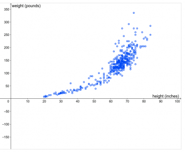
 But actually none of this happens. If I add back the bit of the plot I cunningly hid, we see this:

which suggests a trend line that just might go through zero/zero. The mistake in the first plot was to assume that we could extrapolate beyond the bounds of the observed data. We can't, because the nature of the relationship changes outside the bounds of the data we do know about.

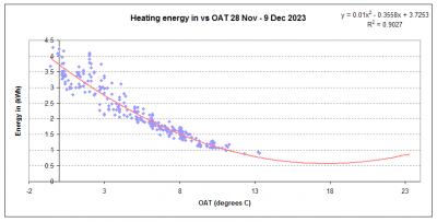
I can achieve similar absurdity by extending my fitted polynomial trend line for heating energy in vs OAT: 

Once the OAT get to around 18 degrees and above, the energy in starts to increase! Extrapolation beyond the observed data is not a good idea!

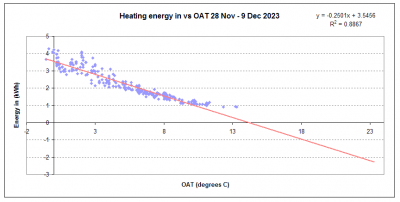
Interestingly, if I change the trend line to a linear one, I get a marginally lower but still very respectable R squared, and the extension stops looking absurd, in fact it is actually credible:

with energy in falling to zero at around 14 degrees OAT. Maybe the linear line is actually the more realistic line? But even this plot becomes absurd if we extrapolate above 14 degrees...so we just don't go there, because it is absurd, in practice trim the chart to exclude the absurd zone. 

Perhaps we need to force the curves, by adding common sense data points clustered around the OAT at which the energy in/out reaches zero, pending getting actual data for mild OATs? But that seems very dodgy to me, even if it makes good logical sense.  

Or we just say we will not extrapolate beyond the bounds of the known, and that way the vampire load never rears its ugly head.

I will take some IR thermometer readings from the PHE inlets and outlets and see if I can get anything useful. 

Edited to correct a rogue image

@cathoderay 

If you think about what is actually happening, the polynomial trend is probably correct, since the heat pump is not the only source of thermal energy within your home. You yourself are probably producing 100W per hour. There is also all the electrical/electronic equipment, and possibly one of the largest, on certain days, is solar gain.

I am getting some interesting results from my spreadsheet, which I hope to post in a day or two.

Posted by: @cathoderay

↑

I wonder if we might be making one of the oldest mistakes in the book, extrapolating beyond observed data. 

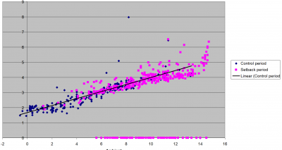
Not really.  The fact that the equation of best fit has a constant in it a fact, and without extrapolation it still means that the data points we actually have are best fit to a curve which has an unexpected and significant constant factor in it that needs to be explained if we are to understand whats going on, because the most simple explanation does not feature such a constant.  Given also that the scattergram of IAT-OAT (corrected for the fabric) vs energy out also has a constant and is a very good fit to a linear equation, there appears, at least for now, to be some considerable evidence that the constant is 'real'.

Posted by: @cathoderay

↑

Or we just say we will not extrapolate beyond the bounds of the known, and that way the vampire load never rears its ugly head.

Except that we still have to explain the offset as set out above and the need to do so is not predicated on extrapolation.

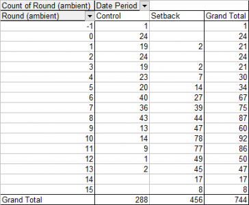
However if we wish to talk about the perils of extrapolation I suggest you take a look at the spread of AATs in the control data vs the spread of AOTs in the setback period.  They are very different indeed.  Here are couple of pivot tables illustrating this.  The first is a frequency table of hourly OAT in 1 degree bins (ignore the meaningless totals)

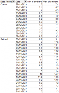
 The second is max and min for each day

The two periods can hardly be described as comparable, so the 'expected', derived from the control period, is effectively based on a small sample of the control data extrapolated to a situation where the diurnal variation is rather smaller!  

Despite this and conscious that we will never have perfect data I remain prepared to believe for now that the energy in during setback appears to be (and thus quite possibly is) lower than would be expected based on the control data to a greater degree than that which can be explained by the savings in heat loss.  With your linear fit the difference is only 11%, but even that is still more than can be explained by the savings in heat loss.  This being the case I think its worth considering possible explanations, albeit bearing in mind that it may be that later data, where is a) more and b) better overlap between the conditions in the 'control' dataset with that in the 'setback' dataset, may yet prove this all to be a wild goose chase .

Posted by: @derek-m

↑

If you think about what is actually happening, the polynomial trend is probably correct, since the heat pump is not the only source of thermal energy within your home. You yourself are probably producing 100W per hour. There is also all the electrical/electronic equipment, and possibly one of the largest, on certain days, is solar gain.

I agree, and there is also the uptick at the left hand end very possibly due to declining COP as Set LWT increases. However, extrapolating beyond the observed data is generally not a good idea, and if it becomes absurd, it is definitely not a good idea! See also a post I am about to publish for some other periods.

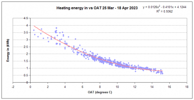
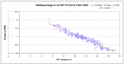
@jamespa - these may be of interest: plots of the periods at the end of the last heating season and the start of this heating season, when there were some higher OAT points:

The R squared values are even better than in the 28 Nov - 9 Dec plot. Perhaps what we see at the right hand ends of the plots is the heat pump standing load? On the second plot, which has some OATs values in the 16 - 17 degree range, I can almost convince myself the line is starting to flat line. 

PS just seem your last post as I was about to publish this, will respond shortly.

Posted by: @cathoderay

↑

The R squared values are even better than in the 28 Nov - 9 Dec plot. Perhaps what we see at the right hand ends of the plots is the heat pump standing load? On the second plot, which has some OATs values in the 16 - 17 degree range, I can almost convince myself the line is starting to flat line. 

Interesting.  It could be standing load or minimum possible output even with cycling (because it probably turns on every so often just to get a sense of its environment) or a combi of the both.  It might be possible to tell from the data whether there was any significant heating energy going to the house at the tail end.  Heat pumps often seem to specify consumption in 3 or so quiescent states, and of course we immediately don't know which it is in!

For what its worth I plotted COP vs ambient during the control and the setback periods.  They were pretty similar, although there did seem to be an odd uptick in the setback results.  My principal motivation for doing this was to try to find out whether the seemingly anomalous results for energy in (specifically that you can apparently reduce the total delivered in a day perhaps by 20% without the house cooling dramatically) are most likely due to a heat pump effect or a house effect (in this case 'house' includes everything beyond the heat pump).  Since the COP curves are apparently similar this points (non conclusively) to a house effect.  

Its still all a bit of a mystery.  It could of course be down to something simple (but not taken into account) like differences in solar gain between the 'control' period and the 'setback' period, or it could yet be a vampire load, secondary heating or something else, or a data artefact on which we are all wasting our time.  Would you be prepared to divulge approximately where you live so we can take a quick look at weather data.

Posted by: @jamespa

↑

The two periods can hardly be described as comparable, so the 'expected', derived from the control period, is effectively based on a small sample of the control data extrapolated to a situation where the diurnal variation is rather smaller!  

Not sure I agree with this, as the control period range spans almost all of the setback period range, meaning the extrapolation is small, and only applies to a very small proportion of setback OATs. But I still think extrapolation is inherently unsound, for the reasons I gave (curve in one place does not necessarily predict the curve in another, unknown, place). Extrapolation is like leaning over the edge of a precipitous cliff, the further you go the more likely you are to suffer a calamitous fall.

But the real answer to all this is more data, and more data is coming in all the time.

Posted by: @jamespa

↑

My principal motivation for doing this was to try to find out whether the seemingly anomalous results for energy in (specifically that you can apparently reduce the total delivered in a day perhaps by 20% without the house cooling dramatically) are most likely due to a heat pump effect or a house effect (in this case 'house' includes everything beyond the heat pump).  Since the COP curves are apparently similar this points (non conclusively) to a house effect.  

I think 'house effect' is very plausible, solid stone walls and solid concrete slab ground floor floors on a small house (high mass to volume ratio), relatively high thermal mass very likely. Plus, when the heat pump is off, it can't do much to alter the heat gain/loss!

Posted by: @jamespa

↑

Would you be prepared to divulge approximately where you live so we can take a quick look at weather data.

South of the M4, but naturally a bit nervous about giving too much away, but that may not be a problem because I already have three hourly weather data from two nearby Met Office weather stations logged in Home Assistant. Here's the last two days data for one of them (also have temps wind speed and direction etc): 

Weather data can be very tricky, especially when it is in text format, you have to work out how to put a number on it (SW 6 veering NW gale 8 occ severe gale 9 in the north backing S 4 for a time later in the west...)  . One of my other recent projects has been to look at how well shipping forecasts predict the actual weather (sounds a bit familiar?) and it is not easy. So far as I know the Met Office did try, just once, in a paper published about a decade ago, and gave up, because it was too difficult to do. No doubt they do it all in house nowadays, and have models that tell them their forecasts are absolutely wonderful. I can tell them they are not, but I would like to be able to prove it! 

Posted by: @jamespa

↑

Posted by: @jamespa

↑

The two periods can hardly be described as comparable, so the 'expected', derived from the control period, is effectively based on a small sample of the control data extrapolated to a situation where the diurnal variation is rather smaller!  

 

 

Not sure I agree with this, as the control period range spans almost all of the setback period range, meaning the extrapolation is small, and only applies to a very small proportion of setback OATs. But I still think extrapolation is inherently unsound, for the reasons I gave (curve in one place does not necessarily predict the curve in another, unknown, place). Extrapolation is like leaning over the edge of a precipitous cliff, the further you go the more likely you are to suffer a calamitous fall.

I think you missed the point.  While the control period covers almost  all the setback range of OAT, it a) has very few data points in much of that range and b) is mostly comprised of days when the diurnal variation was much larger.  Diurnal variation is almost certain to have an effect and you are extrapolating from data comprising days with generally a large diurnal variation to days with generally a small diurnal variation.  Its extrapolation on a different variable, but one which is still important, perhaps particularly so during recovery.

Posted by: @cathoderay

↑

 

But the real answer to all this is more data, and more data is coming in all the time

Indeed

Posted by: @cathoderay

↑

I think 'house effect' is very plausible, solid stone walls and solid concrete slab ground floor floors on a small house (high mass to volume ratio), relatively high thermal mass very likely. 

Its real all right. Bear in mind I including in 'House' everything outside the heat pump itself (ie the rest of the CH system including the PHE).

Posted by: @cathoderay

↑

Plus, when the heat pump is off, it can't do much to alter the heat gain/loss!

Which is why your data, as it stands, is currently unexplained and thus cannot currently be extrapolated to any system or circumstances other than the ones in which it was measured.

Posted by: @cathoderay

↑

Weather data can be very tricky, especially when it is in text format

I think hours of sun is the most interesting figure initially as it might help us get a handle on solar gain, which, depending on your house orientation/window area, may well be the biggest external variable.  Do you have that in your data.  Alternatively there are online sources of solar irradiance by weather station and a random one south of the M4 will almost certainly be good enough

@jamespa

I suspect that some of the wider variation in OAT during the setback data, is probably due to the heat pump being stopped for a lengthy period of time. The raw data consistently shows that some time after the heat pump stops, the OAT reading increases by several degrees, and when the heat pump restarts the OAT reading falls by several degrees, both happening over a short time period so would be unlikely to be a real change in ambient temperature. How would this affect your statistical approach?

We could do with some actual ambient temperature data to compare with the OAT reading provided by the heat pump.

Solar gain, even on cloudy days can be sufficient to affect the heat loss from the building. 

Posted by: @derek-m

↑

The raw data consistently shows that some time after the heat pump stops, the OAT reading increases by several degrees, and when the heat pump restarts the OAT reading falls by several degrees, both happening over a short time period so would be unlikely to be a real change in ambient temperature. How would this affect your statistical approach?

I have no idea how to account for this other than the obvious observation that it is likely to compromise hp performance. 

I'm not sure I'd describe the statistical approach as 'mine', it's data from @cathoderay !  Personally I prefer to account for as many of the material known variables as possible before drawing scattergrams (which I don't much like but sometimes the real world isn't as tidy as I would ideally want). 

However I also have to acknowledge the good correlation between oat and energy in, which, as I refer to upthread, tells us something about the mode in which the system is operating.  For me the question has, as a result, altered from 'why was so much energy apparently saved' to 'why didn't the house cool more? with a side of 'was that much energy _really_ saved?'.  Perhaps your modelling will explain or at least give us further clues where to look.

Posted by: @derek-m

↑

We could do with some actual ambient temperature data to compare with the OAT reading provided by the heat pump.

Solar gain, even on cloudy days can be sufficient, to affect the heat loss from the building. 

Indeed.  ' South of M4' is probably good enough to download some data and @cathoderay tells us he has some independent local data in addition.