Posted by: @jamespa

↑

However others have said that 5C

The lower the DT the higher the flow rate.

The lower the DT on the heating water side, the hotter the average temperature of the heat emitter, so the the heat emitter can be smaller.  You did mention this. = cheaper.

The higher the flow rate the more noise.

The higher the flow rate the higher the heat transfer coefficient in the plate exchanger in the ASHP so the smaller the plate can be = cheaper.

The higher the flow rate the easier it is to get the flow to split equally at t junctions, because the flow will be be in the turbulent regime at all points in the system.  Which makes the pipework installation easier, in theory, therefore faster to install therefore cheaper.

If the plate exchanger is too small it might not be able to condense all the refrigerant so that could lead to energy being wasted over the depressuring valve.

Just some random thoughts

Bob

(my typing is really bad tonight, i hope my ramblings make some sort of sense)

After mulling this over for a while, I have decided to have another stab at answering the question: do the two samples, setback days and no setback days, come from the same population ie there is no real difference between then, they just appear to be different, or from different populations ie in some material way, they are different.

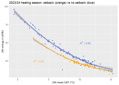
This is the original plot of all the data:

Visually, the two datasets do appear different. Mean daily energy in (kWh) is also different (stats done in R, df_sb is the setback date, df_nosb is the no setback data):

> mean(df_sb$htg_24h_kWh_in)
[1] 21.89719
> mean(df_nosb$htg_24h_kWh_in)
[1] 37.27308

But there is a problem:

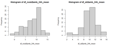
> mean(df_sb$amb_24h_mean)
[1] 10.17582
> mean(df_nosb$amb_24h_mean)
[1] 8.25463

The mean daily ambient temperature was lower during the no setback days. This means we have no way of knowing whether the setback savings happened because (a) the ambient temp was warmer, (b) the setback itself reduced energy use, or (c) a combination of the two (or frankly possibly something else, though that seems unlikely).

The histograms for the mean ambient temps also show they are clearly not the same: 

In an attempt to fix this, I have edited the full data set (the one with both setback and no setback days) to retain only matching pairs, in a manner that might be loosely akin to a matched case control study. I matched on daily mean ambient temperature, keeping only rows where an adjacent opposite setback row had the same daily mean ambient temperature, with a tolerance on 0.1°C. The data ends up looking like this:

2023-12-16T12:01:01	8.1	37.152	0
2023-11-16T12:01:00	8.1	26.957	1
2024-02-28T12:01:01	8.4	33.484	0
2024-03-27T12:01:00	8.4	23.999	1
2023-11-07T12:01:01	8.6	24.874	1
2024-01-04T12:01:00	8.7	33.256	0

The first column is the datetime stamp (days run noon to noon), the second the daily mean ambient temp, the third the total kWh in for the day and the fourth is setback 0 = no, 1 = yes. The first two rows shown are matched on 8.1, the next two rows on 8.4 and the last two rows on 8.6/8.7 (within 0.1°C). This reduced the data set from 199 rows to 85 rows, quite a reduction, but still a usable sample size.

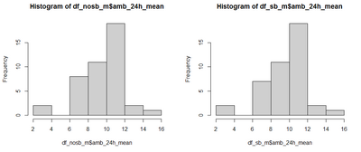
The daily mean ambient temperature are now much closer and the histograms appear pretty much the same (the _m suffix denotes matched data):

> mean(df_sb_m$amb_24h_mean)
[1] 9.685714
> mean(df_nosb_m$amb_24h_mean)
[1] 9.627907

But the difference in mean energy use remains:

> mean(df_sb_m$htg_24h_kWh_in)
[1] 23.62371
> mean(df_nosb_m$htg_24h_kWh_in)
[1] 29.38584

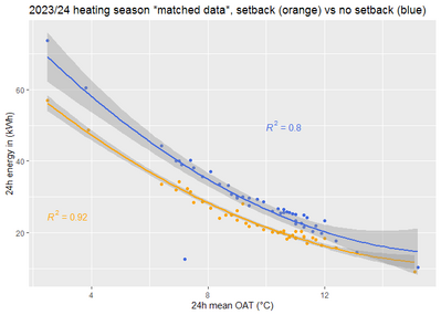
And the scatter plot still suggests samples from different populations:

The net effect of all this is to control for daily mean ambient temperature. Going back to the epidemiological case control study analogy, for each case (a setback day), we have a matched (on daily mean ambient temperature) control (a non-setback day).

We can now run some stats on the matched data set. I have used something called the two sample Kalashnikov-Stalin Kolmogorov–Smirnov test which is a non-parametric (samples do not have to be normally distributed) test for whether two samples came from the same distribution or not. We get a p (probability) value for the null hypothesis that the two samples are drawn from the same population: the lower the p value, the less likely it is that the two samples came from the same population. 

First, lets compare the daily mean ambient temperatures (using R again):

> ks.test(df_sb_m$amb_24h_mean, df_nosb_m$amb_24h_mean)

Exact two-sample Kolmogorov-Smirnov test

data: df_sb_m$amb_24h_mean and df_nosb_m$amb_24h_mean
D = 0.043743, p-value = 1
alternative hypothesis: two-sided

That's encouraging, the matching seems to have worked (p-value = 1, the two data sets have matched ambient temperatures distributions).

Now the daily kWh use:

> ks.test(df_sb_m$htg_24h_kWh_in, df_nosb_m$htg_24h_kWh_in)

Exact two-sample Kolmogorov-Smirnov test

data: df_sb_m$htg_24h_kWh_in and df_nosb_m$htg_24h_kWh_in
D = 0.40975, p-value = 0.001152
alternative hypothesis: two-sided

This is a very low p-value (way way below the conventional 0.05 value, or even the tighter 0.01 value) which tells us that it is extremely unlikely that the samples come from the same population, or, in plain English, they are different.

And in the means (as above) mean anything (these are not normally distributed samples), the difference is not trivial (20%, 23.6kWh with setback vs 29.4kWh with no setback) between the samples looked at. Perhaps we should also look at the median:

> median(df_sb_m$htg_24h_kWh_in)
[1] 20.464

> median(df_nosb_m$htg_24h_kWh_in)
[1] 26.473

Difference 23%, 20.5kWh with setback, 26.5kWh without setback.

The setback running as recorded in this data set appears to use about 20-23% less energy compared to no setback running.

@jamespa - I think this is a fairly robust analysis. If any statisticians out there think otherwise, please do comment!      

@cathoderay 

Im not a statistician but note with interest that the error bands (I presume they are error bands) overlap at OAT>13.  Thats going to mean something at some point in the evolution of this discussion. 

THH I have not doubted for some while that there is a difference in your system between the setback population and the non-setback population, so Im not surprised at further confirmation that this is the case.  Although always very mindful that correlation does not equal causality, presuming that there is a link, albeit possibly indirect/multi-facetted, the question for me is now why?

There are still some known differences between the two sets of conditions for which you haven't, in the most recent analysis, corrected namely the effect of the AIT/OAT sensor and the interior temperature outside setback hours (however that is defined).  Once these are taken out it may well still be the case that the differences exceed that attributable to savings in energy lost from the house, and if so then we need to understand how the balance is made up in order to predict the impact on any system other than yours.

I dont know if your latest technique provides a way to take out the two known differences remaining, if it does then it would be good to do it and if not perhaps we can work on finding another way to do it in the source data and then apply the technique to the result.  This would then give a residual in which the only known effect is the difference in energy lost due to setback and, if the population difference still exceeds that 9which I have a hunch it will) we can think about what else might explain it and the extent to which these other factors may apply elsewhere.

I favour the moving window way to deal with the AIT/OAT sensor.  i was thinking we could apply this to the 'minute' data, but as the figures from the Midea are integers, I dont think we can so will have to rely on the hour data.  The fairly sharp steps when the heat pump switches on/off should still give us a pretty good figure, and from other data we can deduce the 'sign' of the correction to apply.  I will give some more thought to how this could be calculated, but you may well have some ideas

Posted by: @jamespa

↑

Im not a statistician but note with interest that the error bands (I presume they are error bands) overlap at OAT>13.  Thats going to mean something at some point in the evolution of this discussion. 

I'm not a statistician, but I have had to use statistics, mainly but not exclusively in medicine. Yes, they are the 95% confidence intervals, assuming I have understood R's default plotting behaviour correctly. I think the overlap may just be an artefact caused by the fact there are very few data points in that area, sort of a local low (statistical) power means wide confidence intervals.

Posted by: @jamespa

↑

I dont know if your latest technique provides a way to take out the two known differences remaining, if it does then it would be good to do it and if not perhaps we can work on finding another way to do it in the source data and then apply the technique to the result.

I'll see what I can come up with. The essence of the latest analysis is matched controls, if we can find a way of matching on the other variables then progress but inevitably the tighter the matching the fewer the data points remaining, but arguably the more useful they are. That said, I will soon have a whole new data set I can add, from the current 2024/25 heating season, but we will have to bear in mind there have been significant changes, notably opening up all the valves, in the current season.

https://protonsforbreakfast.wordpress.com/2025/12/08/november-2025-heat-pump-analysis-and-setback-evaluation/
Michael de Podesta has attempted to quantify this and I’m pleased to read that for his house the better documented conclusions are in cold weather it could COST more to use setbacks. Our house definitely seems to take too long to recover (ie beyond the cheap period plus battery capacity) to make it worth while. I speak as a continuous fiddler who isn’t good at writing things up.

There are 2 issues here. The Topic is Setback Savings but the vast majority of the discussion has been around ENERGY usage. However with ToU tariffs increasingly used by the majority of owners of heat pumps as well as owning other tech invluding batteries, EVs etc its important to consider COST as well. Some people may feel energy usage is their sole interest - that is fine but not my choice.

Obviously massively complex to analyse or compare if using tariffs like Agile. Complex if using batteries in the mix or on tariffs like Go/Intelligent Go.

In my case I'm on Intelligent Go with 7p overnight rate that i use to fill batteries as well as heat home. With such a cheap rate it makes sense to BOOST heating by say 1 degree overnight to lower daytime demand as the thermal mass will be helped. I have no doubt that works for me even if overnight outside temperatures are low - reducing SCOP.

So my setback is effectively a daytime setback from higher night temp.

No one answer that fits every scenario or usage. And i accept some people may consider it wasteful in energy terms. 

Posted by: @tim441

↑

In my case I'm on Intelligent Go with 7p overnight rate that i use to fill batteries as well as heat home. With such a cheap rate it makes sense to BOOST heating by say 1 degree overnight to lower daytime demand as the thermal mass will be helped. I have no doubt that works for me even if overnight outside temperatures are low - reducing SCOP.

Absolutely.  I tend to call this a set forward.  I also have a similar night-time tarrif, I don't bother with a set forward but I do my DHW cycle at night which is the least efficient time to do it but also the cheapest.

Posted by: @tim441

↑

No one answer that fits every scenario or usage. And i accept some people may consider it wasteful in energy terms. 

Also absolutely to the first.  The second is interesting.  Unfortunately the correlation, at least in the short term, between energy price and carbon footprint appears to be weak, otherwise there would be a very good case for saying that using when its cheap is also when its greenest so waste isn't the issue.  With a simple tarrif like cheap overnight rate and  simple response like your set forward it would be interesting to compare the average carbon intensity by time of day.  I cant lay my hand on that statistic but it must exist somewhere!

Posted by: @jamespa

↑

With a simple tarrif like cheap overnight rate and  simple response like your set forward it would be interesting to compare the average carbon intensity by time of day.  I cant lay my hand on that statistic but it must exist somewhere!

OK so I resorted to AI.  here is what duck.ai says

Morning Peak (6 AM - Noon): 80-100 gCO₂/kWh.

Increased contribution from renewables right after sunrise, particularly solar.

Afternoon Dip: 70-80 gCO₂/kWh.

High solar output significantly reduces reliance on fossil fuels.

Evening Peak (5 PM - 9 PM): 120-140 gCO₂/kWh

Increased use of gas-fired plants to meet higher demand, leading to higher carbon emissions.

9 PM - Midnight: 120 - 150 gCO₂/kWhGas

Higher emissions due to increased gas generation; variability from wind

Midnight - 6 AM: 80 - 100 gCO₂/kWh

Lower demand leads to reduced intensity; renewables become more prominent

Make of that what you will, basically it says use energy at night or during the afternoon if you want it to be carbon-efficient.

@jamespa yes, i should add i also schedule DHW heating for night time. Most of the time we use less than full tank per day so heat to 50deg at cheap rates. Daytime boosting to just 40deg if/when needed. 40 deg is still hot enough to require addition of a little cold water.

The other advantage of scheduling this way is that the heat pump is worked at home heating without interruptions for DHW

@judith — it's an interesting analysis (as his analyses usually are) and he does in fact do something similar to what I have done, though he uses a different language (counterfactual, a long modern word I personally don't like, whereas I tend to use observed (with a setback) vs expected (without a setback). We are both trying to answer the same question: given a period of setback running, how much energy would we have used if we hadn't had a setback? The best way to answer this question is empirically, by having two periods that are otherwise identical, and only differ in that one uses setback running, the other continuous running. Tot up the energy use for each period, and you have your answer. The problem is that in the real world it is almost impossible to run that experiment (nature is so obtuse!), though over time I am building up a data set that may just have periods that are similar enough, but haven't got there yet. As a result we have to estimate what the energy use would have been, rather than measure it.

The starting point for these calculations are the plots of OAT vs energy use, since the OAT is a major determinant of heat loss, and so energy use. A spreadsheet will give you a trend line and equation, and you can use that equation to calculate the (mean) energy use for any OAT in the range you have (ie be wary of extrapolation). This should then give you the energy you would have used in any setback hour had the heating been on rather than off. We already have the observed use during the setback (0kWh), We now also have the expected use, had we not had the setback. The saving is the observed use during the setback minus the expected use without the setback, and it will be negative because it is a saving (you used less energy).

So far so good, but then it suddenly gets more complicated: what happens during the recovery period? Given a normal low and slow heat pump will take forever to reheat the property back to its desired temperature, we end up putting in more heat during the recovery (I use my auto-adapt script to do that), and on top of that the higher flow temperature means a lower COP, such that there are two things that increase the energy use: the higher flow temperature itself, and the lower COP caused by having that higher flow temperature.

But in reality things are not that complicated, because with sufficient monitoring, we have a record of what the energy use is during the recovery period (the observed value), and once again, we can estimate the expected use had there not been a setback, using the method described above, and once again do our observed mins expected calculation. This time the result will normally be positive, because we end up using more energy during a recovery than we would have use with steady running. By summing the hourly energy use with and without setback over longer periods (weeks, months) we should get an answer to our question, do setbacks reward us with savings?

I will do the analysis on my data for November and post the results here once the analysis is done. In the meantime, I still have these charts (posted above, repeated here) which continue to bug and intrigue me, because they do appear to show a saving:

Posted by: @tim441

↑

However with ToU tariffs increasingly used by the majority of owners of heat pumps

They are being increasingly used, but not yet by the majority of heat pump owners, and the same goes for ancillary generation and storage. According to Ofgem (April 2025, see page 21), only 2.3% of consumers in the domestic retail market (Ofgem's windy why use one word (homes) when you can use six (consumers in the domestic retail market) - where do these twerps learn their English?) are on ToU tariffs, and that appears to be mainly driven (sic) by EV use. Even with a large percentage year on year increase, that number is still going to stay small for some considerable time, unless something else changes.

Posted by: @tim441

↑

its important to consider COST as well. Some people may feel energy usage is their sole interest - that is fine but not my choice.

I agree. The reason I, and I suspect others, focus on energy use is because it removes the complexities of different tariffs, but for the individual, what they want to know is how much their heating is costing them, and that of course depends on their tariff. With ToU tariffs it get even more complicated, because you need to know the unit rate for every hour, to determine the cost. That's why it is simpler to do the basic analysis for energy use, and then turn that into costs once you have the hourly tariff rates.

And indeed it does get even more complicated when a consumer in the domestic retail market, as we are now known, starts banking energy at a cheap over night rates, either in a battery or the property's fabric. They may well use more energy, while at the same time their overall costs may be lower.

As you say, no one answer that fits every scenario or usage. We all end up having to do our own cost calculations. based on our tariffs, and how we run things.   

Posted by: @jamespa

↑

OK so I resorted to AI. 

Don't do it! Every time you use AI, a few more of your little grey cells die. Plus the answer looks very questionable to me. 

Posted by: @cathoderay

↑

Don't do it! Every time you use AI, a few more of your little grey cells die. Plus the answer looks very questionable to me. 

Fair enough, I wanted some quick insight and didnt know where to look for the data other than the obvious which i had already tried.

Having got the result I thought about it (hopefully reviving some brain cells) and realise that the answer is probably either averaged over an unspecified time or for the whole year, and what we want is an average over the heating season.   

Sadly my brain cells are probably being slowly pickled due to an unhealthy appreciation of hopped water